Markovian package - Assessing risk using Markov graphs

Creating a Markov graph is easy using the intuitive graphical interface into which the different states of the system can be entered and connected via transitions. For each state on the graph, users can indicate whether or not the system is available. For production efficiency studies, users can indicate the efficiency of the system in each state. Lastly, when the transition rate between states has been entered, the Markov graph is complete, and calculations can then be performed.

The Markov module provides a wide range of results:

• The probability of being in a given state.
• The cumulative sojourn times in each state.
• The availability/reliability of the system.
• The failure rate and Lambda Equivalent for the system over time.

• • Calculation of system efficiency: When a state in the graph indicates that the system is available, the efficiency of the system in this state can be specified. This means that downgraded states can be taken into account and production availability calculations performed.

• Value over time :  It is useful to know the probability of a system being in a specific state at the end of a task over a given operating period, but knowing how it has evolved over time is even better.

The figure above shows an example of a graph produced for a system consisting of 3 components. Each line represents the probability of the system being in one of the 4 states below (at t=0, a component has failed):
- State1: the 3 components are working. 
- State2: 1 component has failed. 
- State3: 2 components have failed.
- State4: 3 components have failed.

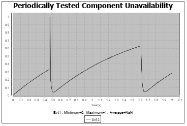
A system will not adhere to the same model throughout its life cycle. It may need to undergo tests or repairs during which time the system would be represented by a different Markov graph. These different phases of a component’s lifetime can be modeled in the Markov module, which can be used, for example, to display the availability of a system that is periodically tested, taking into account a large number of parameters: test duration and efficiency, reconfiguration errors, etc.

Markov graphs can be used with all the GRIF Boolean module (Tree, ETree, BFiab, Reseda, SIL and Risk) to describe a component failure.

• Option to automate calculations (batch runs) and draw variations for sensitivity analysis.
• Results are stored in the document and can be exported in a variety of formats (csv, XML, Excel, etc.).
• Results can be viewed as line graphs, pie charts or histograms.
• Printing in PDF vector format produces high-quality images and the files are small enough to be sent by email, even if the document contains hundreds of pages.
• External files (PDF certificates, system images, etc.) can be added to the document and incorporated into the full report.
• Interaction with the operating system: option to copy/paste either to or from word processing software, spreadsheets, or presentation tools.